Apply a Quick Conditional Formatting Color Scale

Microsoft Excel provides you with several conditional formatting rules for color scales that you can apply with a quick click. These include six two-color scales and six three-color scales. Select the cells that you want to apply the formatting to by clicking and dragging through them. Then, head to the Styles section of the ribbon on the Home tab. Click “Conditional Formatting” and move your cursor to “Color Scales.” You’ll see all 12 options in the pop-out menu.

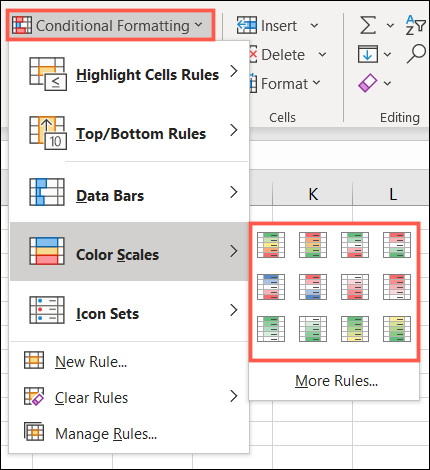
As you hover your cursor over each one, you can see the arrangement of the colors in a screen tip. Plus, you’ll see the cells that you’ve selected highlighted with each option. This gives you a terrific way to select the color scale that best fits your data.

When you land on the scale that you want to use, simply click it. And that’s all there is to it! You’ve just applied a color scale to your data in a few clicks.

Create a Custom Conditional Formatting Color Scale

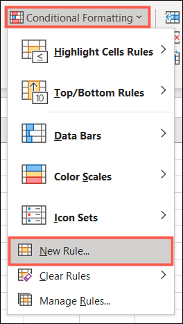
If one of the quick rules above doesn’t quite capture how you want your color scale to work, you can create a custom conditional formatting rule. Select the cells that you want to apply the scale to, go to the Home tab, and choose “New Rule” from the Conditional Formatting drop-down list.

When the New Formatting Rule window opens, select “Format All Cells Based on Their Values” at the top.

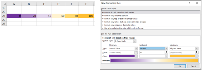
The Edit the Rule Description section at the bottom of the window is where you’ll spend a bit of time customizing the rule. Start by choosing 2-Color Scale or 3-Color Scale from the Format Style drop-down list. The main difference between these two styles is that the three-color scale has a midpoint, whereas the two-color scale only has minimum and maximum values.

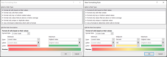
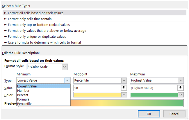
After selecting the color scale style, choose the Minimum, Maximum, and optionally, the Midpoint using the Types drop-down lists. You can pick from Lowest/Highest Value, Number, Percent, Formula, or Percentile. The Lowest Value and Highest Value types are based on the data in your selected range of cells, so you don’t have to enter anything in the Value boxes. For all other types, including Midpoint, enter the Values in the corresponding boxes.

Finally, click the Color drop-down buttons to select your colors from the palettes. If you want to use custom colors, select “More Colors” to add them using RGB values or Hex codes.

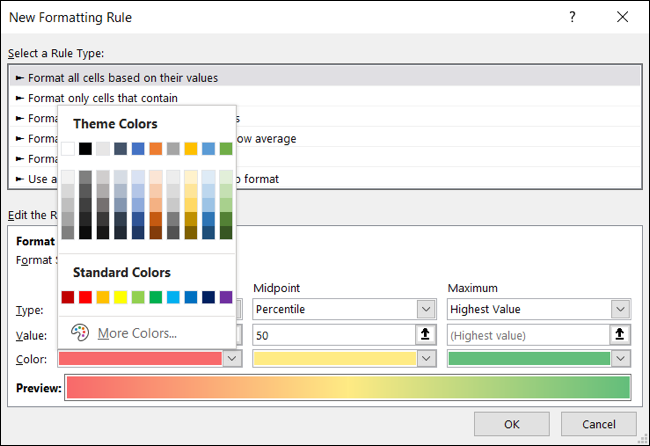
You’ll then see a preview of your color scale at the bottom of the window. If you’re happy with the result, click “OK” to apply the conditional formatting to your cells.

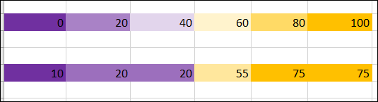
The nice thing about a conditional formatting rule like this is that if you edit your data, the color scale will automatically update to accommodate the change.