Situatie
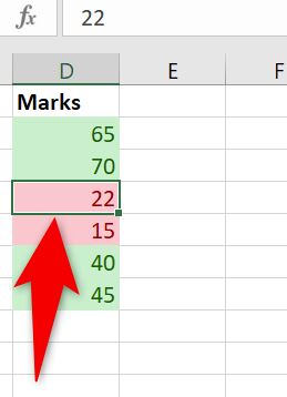
Using Microsoft Excel’s sorting feature, you can sort your cells that are either manually colored or conditionally colored by their color. This works for multiple colors and we’ll show you how to implement it in your spreadsheets. With the feature, you can place the cells containing a specific color at the top or the bottom of the list. For example, you can place all your green-colored cells at the top while keeping all the red ones at the bottom.
Solutie
Sort Data by Cell Color or Font Color in Excel
- To start sorting, open your spreadsheet with Microsoft Excel. In your spreadsheet, click any cell in your dataset.
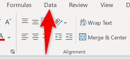
From Excel’s ribbon at the top, select the “Data” tab.
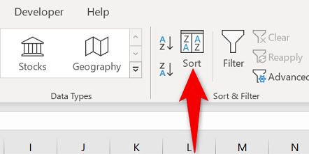
On the “Data” tab, from the “Sort & Filter” section, choose “Sort.”
- A “Sort” window will open. If your dataset has headers, then in this window’s top-right corner, enable the “My Data Has Headers” option.
- Click the “Sort By” drop-down menu and select the column whose data you want to sort. From the “Sort On” drop-down menu, if you want to sort your cells by their background color, choose “Cell Color.” To sort cells by their font color, select “Font Color.” We’ll go with the former option.
- Next, click the “Order” drop-down menu and choose the color you want to keep at the top or at the bottom. Next to this drop-down, click another drop-down and select where you want to place the cells containing the selected color. Your options are “On Top” and “On Bottom.”
- If you have three or more color cells in your dataset, feel free to add another sorting level by clicking “Add Level” at the top of the “Sort” window.
- Finally, at the bottom of the window, click “OK” to apply your changes.

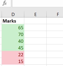
Back on your spreadsheet window, you will see your cells sorted by their color.
Leave A Comment?