How to Use Relative References in Excel

In the example shown here, you can see how much the person has spent on each item in each month. What they now want to do is work out the total spend for each month.

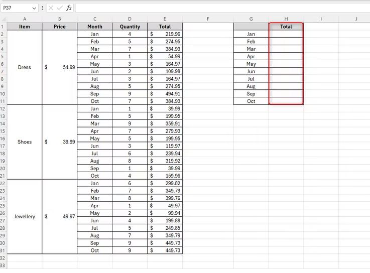
First, click the cell where you want the first calculation to be made (in this case, H2), and type the formula to create this calculation. In this example, you would use the following formula:

=SUM(E2+E12+E22)


This has now referenced cells E2, E12, and E22 within the calculation, adding them together. 
This is a relative reference—the formula in cell H2 has referenced the cells that are three columns to the left (E2),
three columns to the left and ten rows down (E12), and three columns to the left and twenty rows down (E22), respectively.
Now, if you were to copy and paste that same formula elsewhere, 
it would pick up the values that are in the same relative positions to where you paste it. 
You can also use Excel's Autofill to complete the rest of your data with the same relative reference.

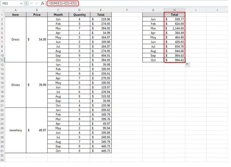
As you can see here, the formula in cell H11 is:

=SUM(E11+E21+E31)

This is because the relative reference is placed nine rows down from where it was originally. Now, rather than typing the formula for each month, you only have to type it once and then apply the same relative reference wherever you want on your Excel worksheet.

How to Use Absolute References in Excel

In this example, the company accountant wants to work out how much to pay the employees based on the number of hours they have worked and a fixed hourly rate.

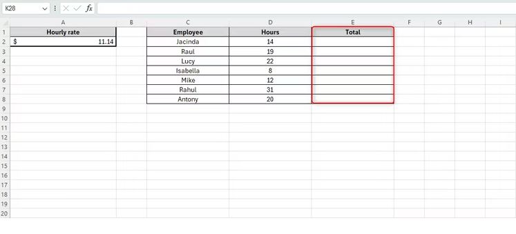
Start by clicking the cell where you want the first total to be calculated (in this case, E2), and begin to type the appropriate formula. In this example, the accountant wants to multiply the hourly rate in cell A2 by the total hours worked by Jacinda in D2.

=SUM(A2

However, if we use a relative reference here, when we apply the formula to the other employees’ totals, the formula will reference cell A3 for Raul, A4 for Lucy, and so on, meaning you will not get the results you want.

So, we need to make sure that Excel continues to refer to the correct cell, which, in this case, is A2. To do this, you need to insert the dollar symbol before each part of your reference:

=SUM($A$2

This now tells Excel that if we use the same formula elsewhere, A2 will always be referenced.

You can now complete your formula. In this case, it will be as follows:

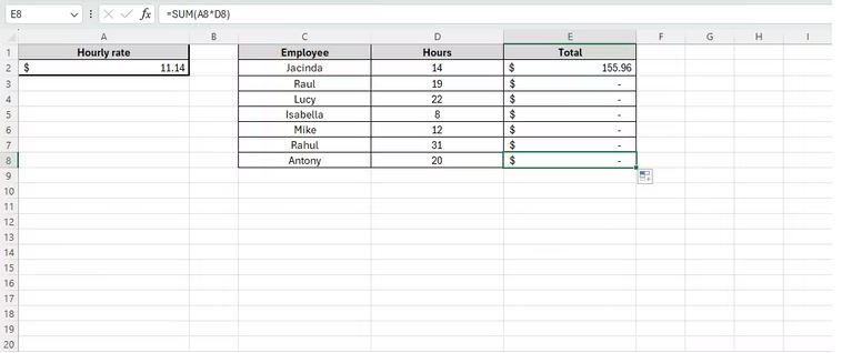
=SUM($A$2*D2)

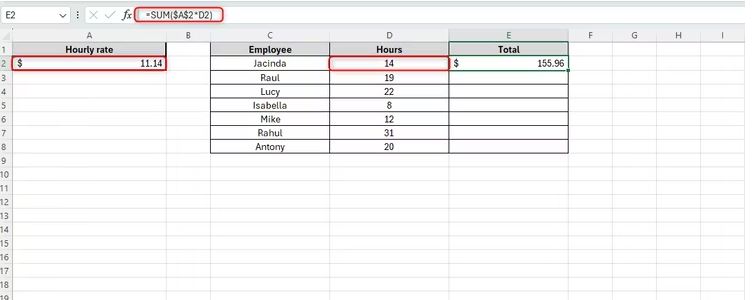
Note how the second part of the formula (D2) does not use an absolute reference. This is because we want to multiply cell A2 by each employee’s respective hours, so that needs to be relative to each person’s hours in column D.

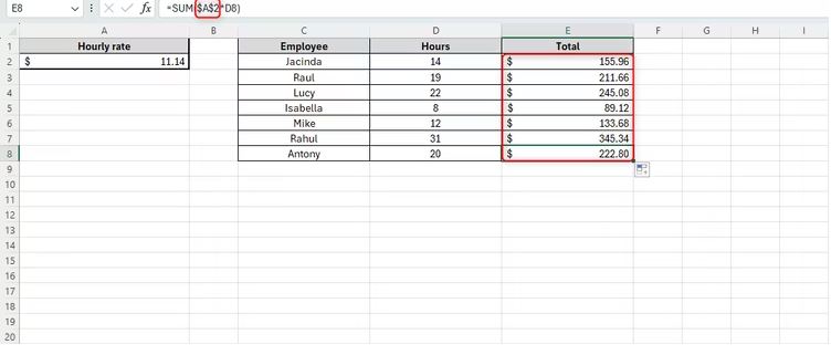
You can now apply the formula to the other cells by copying and pasting it or using Excel’s AutoFill function, knowing that cell A2 is referenced absolutely.

How to Use Mixed References in Excel

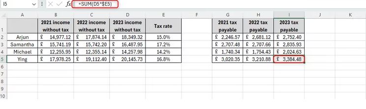
There may be occasions when you need to lock the row but not the column within your formula, or vice versa. For example, in this case, the accountant wants to work out how much tax each employee has to pay based on their individual tax rates.

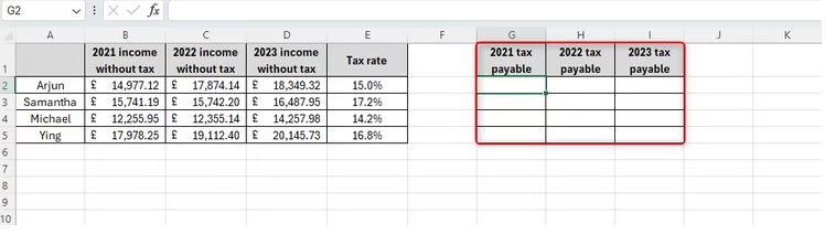
Therefore, we need to lock the values in column E (the tax rates), but not the rows, as they are different for each employee, and not the references to the years, as they need to be adaptable.

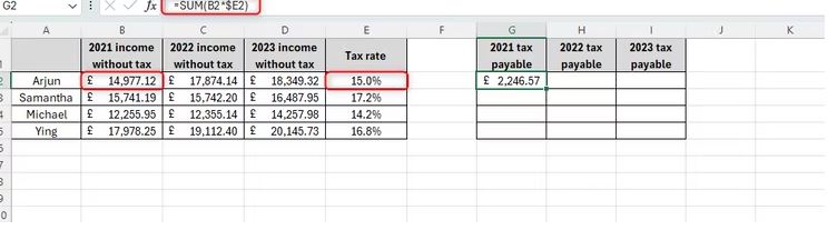
Click the cell where you want the first calculation to be made (in this case, cell G2) and input your formula. In the example above, the accountant wants to begin by working out Arjun’s 2021 tax payable, so they would type the following formula:

=SUM(B2*E2)
We now need to lock column E. If we were to AutoFill to the right without 
the formula being amended, it wouldn't correctly calculate Arjun's 2022 tax payable; while it 
would accurately pick up the correct yearly income totals (because we are not locking cell B2), 
the formula would also reference cell F2. To do this, add a dollar symbol before the reference to column E in your formula:

=SUM(B2*$E2)
We don't want to use an absolute reference here because that would mean 
that, when we work out the tax payable for the other employees, Arjun's tax rate would be used 
instead of each employees' individual rates. In essence, locking only column E means that we will stay on 
the tax rates but can relatively adjust to each person's different rates.

We can now use the AutoFill function to complete Arjun's tax payable totals, 
knowing that column E will remain locked in our calculations, whilst the totals for each year will move relative to where the formula is placed.

Because we have locked column E but left the rows relative within our formula, 
we can confidently complete the remaining employees' totals based on their individual tax rates.
 Remember, you can click any cell within your results and see the formula in the formula bar to check the correct cells are referenced.